The Ugly Professor? Professor evaluations vs physical appearance
by L. Mark Coty
The data are gathered from student evaluations for 463 courses taught by a sample of 94 professors from the University of Texas at Austin. Also, six students rate the professors' physical appearance. The result is a data frame where each row contains a different course and each column has information on the course and the professor who taught that course.
GitHub repository here. Run the notebook.
Purpose:As a long -time college professor, I was immediately interested when I encountered this recent dataset containing the results of a study intended to provide insight into the perceived appearance of professors and the quality of the course evaluations they received from their students.Upon closer inspection, there seemed to be enough data to ask and possibly answer such questions as:1. Do professors with higher "beauty" ratings also tend to receive higher evaluations, as instructors, by their students?2. Do males or females get higher evaluations from their students?
Overview:I began with a dataset containing student evaluations for 463 courses taught by a sample of 94 professors from the University of Texas at Austin. Also, six students not in the courses rated the professors' physical appearance. The result is a data frame where each row contains a different course and each column has information on the course and the professor who taught that course.The GitHub repository containing all of the work can be found here.
The Content and Nature of the Data:
The columns in the dataset and their types are as follows:
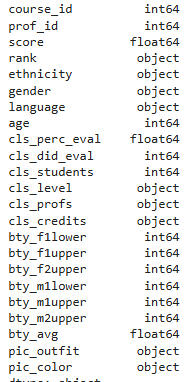
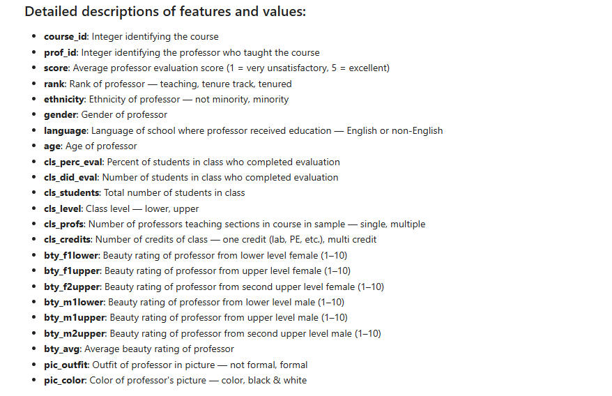
Explanation of non-obvious columns and values:
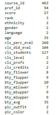
The number of unique values in each column are as follows:
To Visualize the Categorical ("object") Data, We Can Examine Their Percentage Bar Graphs:
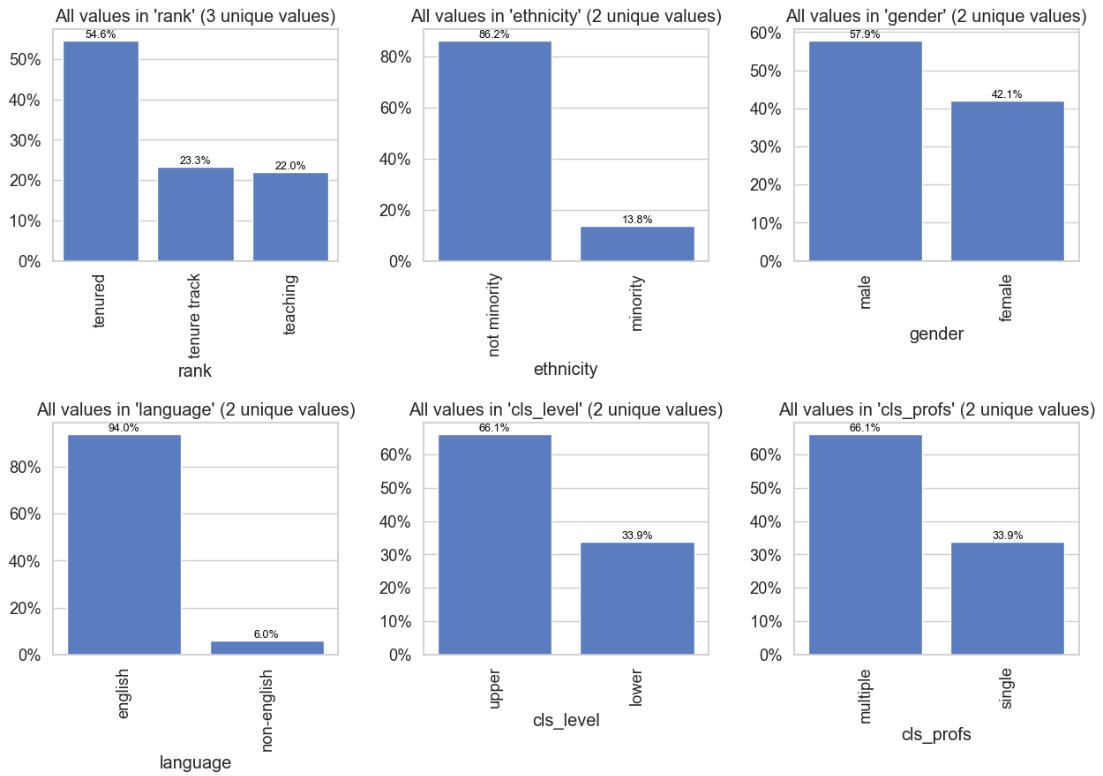
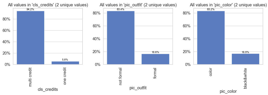
Observations from the above graphs:
There are more tenured professors than the other categories combined.
Only about 14% of the professors are minority.
Males exceed females by about 15%.
Only 6% of the professors attended non-English speaking institutions.
About 2/3 of the classes were upper-level.
About 2/3 of the courses had multiple professors teaching them.
Almost all courses were multi-credit.
Only about 17% of the professors were formally dressed in their photos.
Only about 17% of the photos were in black-and-white.
Based on this, it seems that 'language' and 'cls_credits' might well be dropped from the rest of the analysis. We will do that.
Let's examine histograms of the numerical columns:
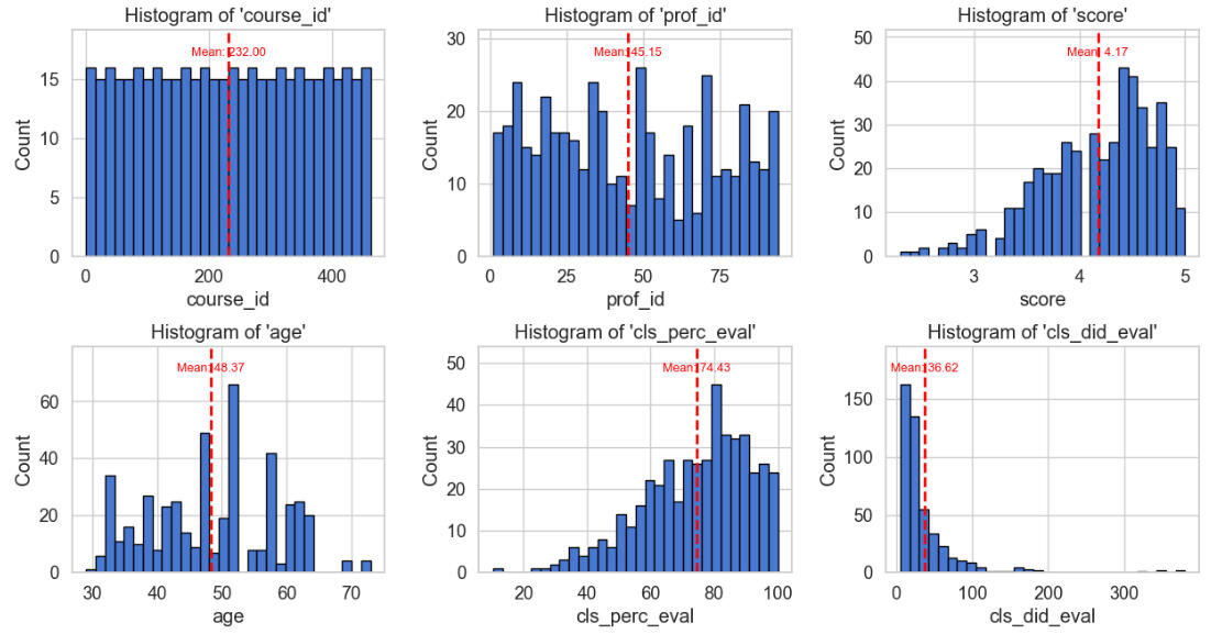
Observations on the above histograms:
Course ID is uniformly distributed, and so not very informative. It can be dropped.
Prof_ID is essentially categorical/nominal, since it merely identifies the instructor.
Score shows a mean attractiveness of 4.17, with a strong left-skew. This is an important number.
Age shows a mean of about 48, and is quite irregularly distributed.
About 74% of students completed professor evaluations, very left-skewed shape.
About 37 was the mean number of students in a class that did the evaluations, very right skewed (could be due to class sizes).
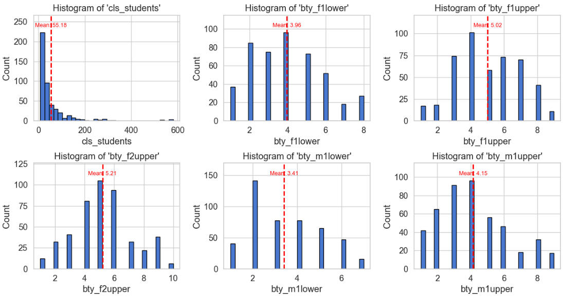
55 was the mean class size, again very right-skewed, as in the previous case.
The mean beauty ratings given by each of the six judges were:
Lower-level female: 3.96
Upper-level female 1: 5.02
Upper-level female 2: 5.21
Lower-level male: 3.41
Upper-level male 1: 4.15
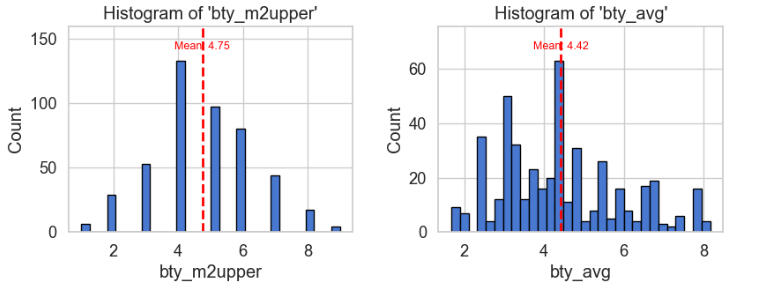
Upper-level male 2: 4.75
Overall average beauty rating: 4.42
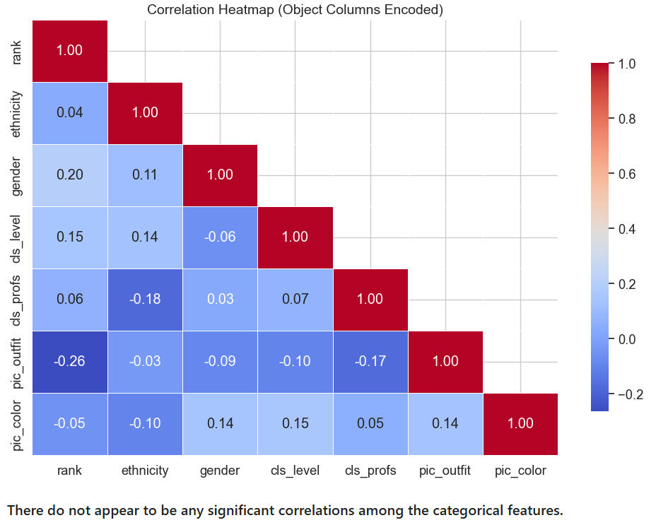
Let's look at a heatmap of the categorical columns:
Let's look at a heatmap of the numerical columns:
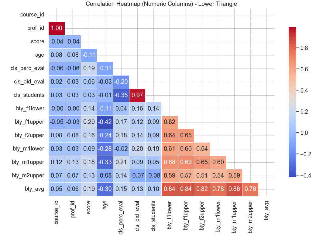
Observations on the above heatmap:
* The values at or near 1 can be disregarded: They merely reflect that courses match professors and that class size is nearly perfectly correlated with the number of evaluations done.
* It is interesting that the upper-level female judge's ratings correlate fairly strongly (negatively) with professor's age (-0.42).
* As for the orange tiles, they merely reflect the general agreement among the judges. Note that the 2nd upper-level male judge has the weakest correlation with the other judges, though not by much.
We will drop the columns of the six individual judges (bty_f1lower, etc.), since the focus of this analysis is the judgment of the students "en masse", and as can be seen in the bottom row, the average rating from each individual judge correlates very strongly with the overall rating, "bty_avg".
We now have a compact enough dataframe to create a heatmap of all the features, categorical and numeric:
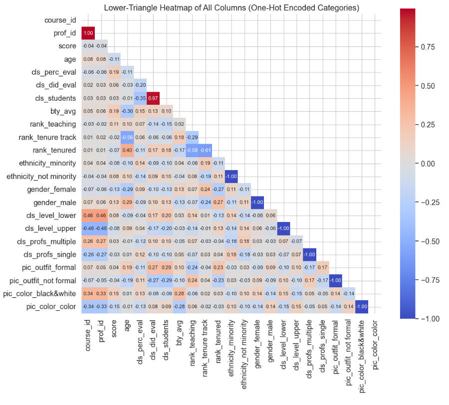
Observations on the above heatmap:
* There are few noticeable strong correlations, aside from the trivial ones in which binary columns have -1.00 between the two values, or the two values of 1.0 and 0.97, which were discussed in the previous heatmap.
* The correlations between age and tenure status are also to be expected and do not indicate anything significant about the data.
Let's employ some classifiers to see if we can predict evaluation "score" (the target) based on:
Ethnicity
Gender
Age
Beauty_avg
Pic_outfit
Pic_color
since these are features that are most visible and relevant in judging looks.We'll use SVC, Decision Tree, Random Forest, XGBoost, and Logistic Regression models.
We will use the mean of 4.17 for the target "score" as the cutoff, seeing if we can predict "below mean" vs "mean or higher" based on the features. We'll use a holdout evaluation (25% test set) with Accuracy, Precision, Recall, F1, ROC-AUC, and confusion matrix counts. We'll also include a 5-fold cross-validation summary with mean metrics.
The results of employing these classifiers are summarized below:
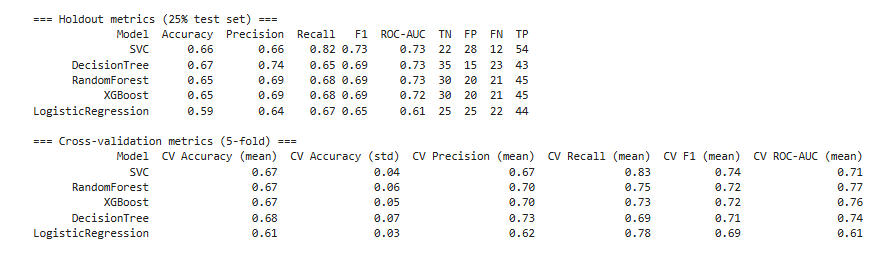
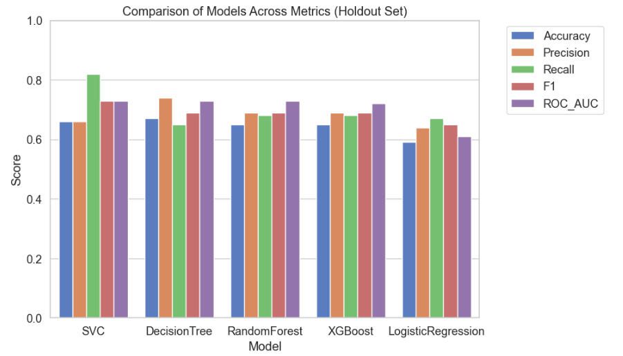
Observations on the above table of metrics:
All models are in the 0.65–0.68 accuracy range (except Logistic Regression at ~0.59–0.61).
This suggests the problem is not trivial, but also not highly separable by these models with the current features.
SVC: Highest recall (0.82 test, 0.83 CV), meaning it catches most positives, but at the cost of false positives (low TN).
Decision Tree: Highest precision (0.74 test, 0.73 CV), meaning when it predicts positive, it’s more likely to be correct, but it misses more positives (lower recall).
Random Forest / XGBoost: More balanced between precision and recall (~0.69 each).
If missing positives was costly, SVC would be better.
If false alarms were costly, Decision Tree would be better.
For a middle ground, Random Forest / XGBoost would be best.
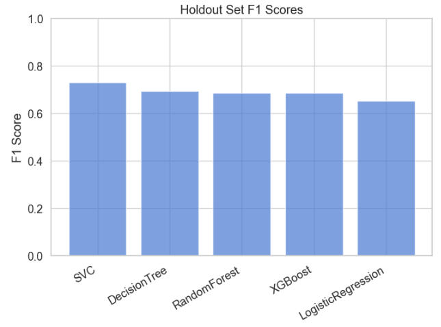
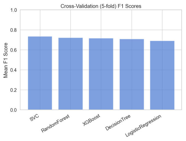
Below are plots of F1 and Mean F1 for the models:
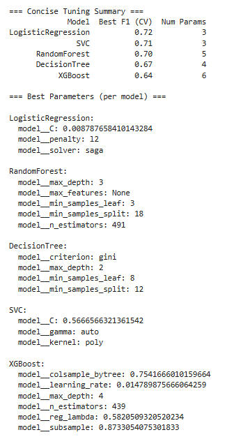
Let's try tuning the hyperparameters using RandomizedSearchCV.Here are the results:
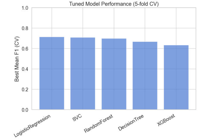
Let's look at a graph of the post-tuning results:
And here is a graph comparing all the models across metrics:
Now let's focus on the F1 score before and after tuning:
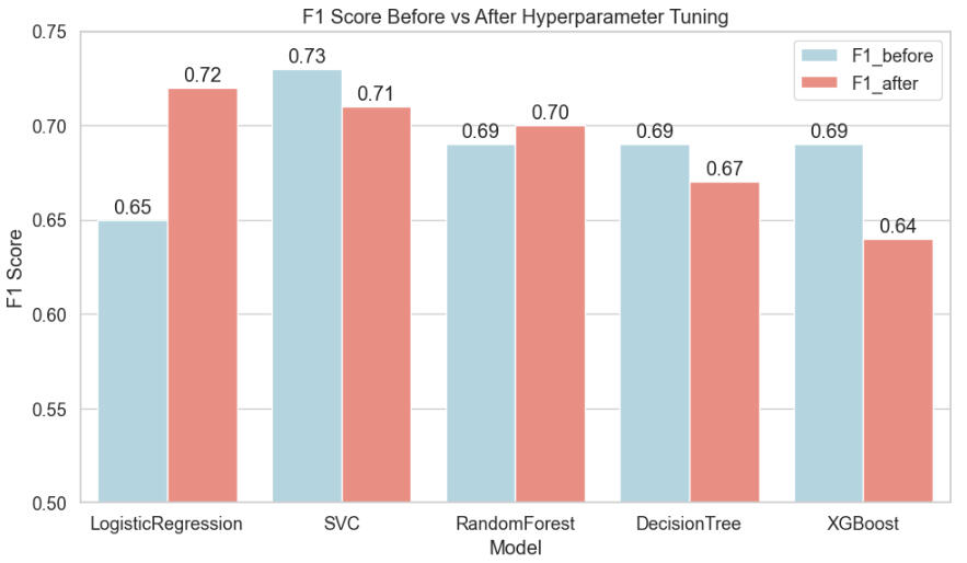
Interpretation of the above plot:
Logistic Regression: biggest gain from tuning → strong regularization made a big difference.
SVC: small decrease in F1 → tuning shifted the balance of precision/recall slightly.
Random Forest / Decision Tree: minor improvements or small drop → tuning mainly prevented overfitting rather than boosting F1.
XGBoost: decreased F1 → tuning made it very conservative, likely underfitting.
F1 performance after tuning:
Logistic Regression: Best F1 = 0.72 → surprisingly strong for such a simple model, especially given that before tuning it was ~0.65. This suggests regularization (C≈0.009) helped significantly.
SVC: Best F1 = 0.71 → slightly lower than LR, still high recall/precision balance.
Random Forest: Best F1 = 0.70 → fairly close to SVC/LR, indicating the ensemble adds stability but not a huge F1 boost.
Decision Tree: Best F1 = 0.67 → modest gain from tuning, but limited by simplicity (max_depth=2).
XGBoost: Best F1 = 0.64 → underperformed relative to expectations; tuning pushed it to a very cautious/low learning rate configuration, likely underfitting.
Conclusion: Simpler models (LR, SVC) dominate in F1 after tuning, probably because the dataset is small and simpler models generalize better.
Hyperparameter tuning overview:
Logistic Regression:
C ≈ 0.0088 → very strong regularization (small C), prevents overfitting.
SVC:
C ≈ 0.567, kernel = poly, gamma = auto → moderate regularization, polynomial kernel may help capture some nonlinearity.
Random Forest:
max_depth = 3, min_samples_split = 18, min_samples_leaf = 3 → very shallow trees, cautious splitting → again, likely avoiding overfitting on a small dataset.
n_estimators = 491 → plenty of trees to stabilize predictions.
Decision Tree:
max_depth = 2 → extremely shallow, basically a high-bias model.
min_samples_leaf = 8 → ensures leaves have enough data → reduces variance.
XGBoost:
learning_rate ≈ 0.015, max_depth = 4 → very conservative boosting; almost certainly underfitting.
All tuned models are very conservative (shallow trees, strong regularization, low learning rate). This indicates the dataset is small, noisy, or both. Aggressive models likely overfit.
Simpler models perform best, which is consistent with the CV F1 scores: LR > SVC > RF/XGBoost > DT.
XGBoost underperforms because the low learning rate combined with shallow depth limits its ability to capture complex patterns.
Bottom line: Logistic Regression turns out to be strong and interpretable.
Let's plot the average score on the professors' evaluations over their ratings on the beauty scale, shaded by gender.
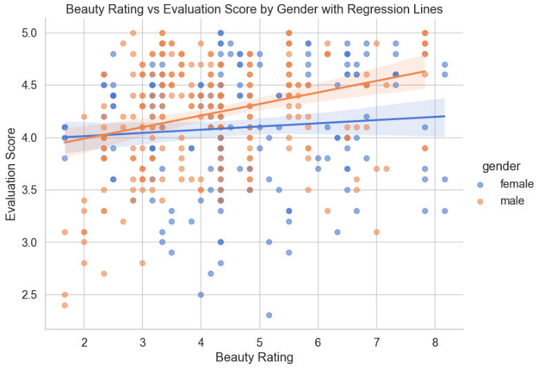
A quick glance at the above graph appears to show that female professors' evaluations are less dependent on their beauty ratings than are their male counterparts'. Let's check the metrics of the lines and the regression:
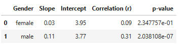
Conclusions from the linear regression models:
Slope:* Female: 0.03 → For each 1-unit increase in beauty rating, average evaluation increases by only 0.03 points (very small effect).
* Male: 0.11 → For each 1-unit increase in beauty rating, evaluations increase by 0.11 points (larger effect).
* Interpretation: Beauty has a stronger positive relationship with evaluation scores for male professors.Intercept:* Female: 3.95, Male: 3.77 → The baseline evaluation score when bty_avg = 0. This is not meaningful since beauty ratings don’t really go down to 0, but it anchors the regression lines.Correlation:Female: 0.09 → very weak correlation (close to zero).
Male: 0.31 → moderate positive correlation.*Interpretation: Male professors’ scores show a more noticeable upward trend with beauty ratings, whereas female professors’ scores barely change with beauty.p-value:*Female: 0.2348 → not statistically significant (greater than 0.05). The slope could easily be due to chance.
*Male: 2.0 X 10⁻⁷ → highly statistically significant. The relationship is very unlikely due to chance.
Bottom line: Beauty significantly predicts evaluations for male professors, but not for female professors.In other words, for female professors, the line is nearly flat, and the relationship between beauty and teaching evaluations is weak and statistically non-significant. So beauty doesn’t predict evaluations meaningfully.For male professors, the slope is steeper, correlation is moderate, and the relationship is statistically significant. This suggests that male professors perceived as more attractive tend to get better evaluations.
Hypothesis Testing:
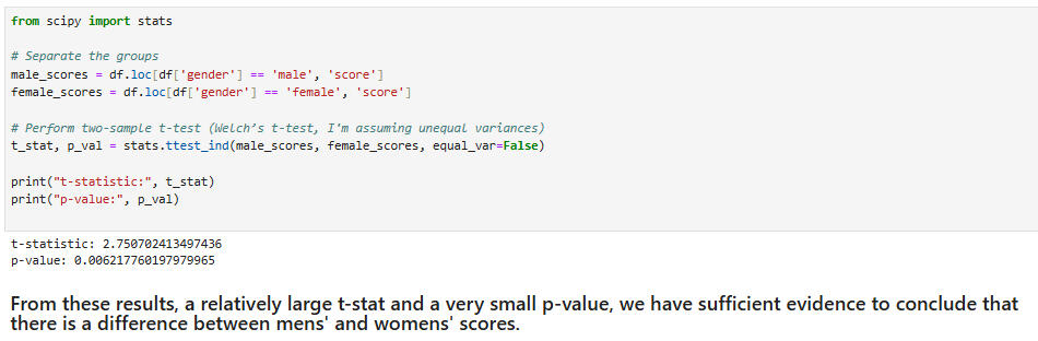
Let's perform a 2-sample t-test to see if the difference between mean male and female evaluation scores is significantly different.So:(H₀): Male and female professors have the same mean evaluation scores.
(H₁): Male and female professors have different mean evaluation scores.
Let's examine their boxplots:
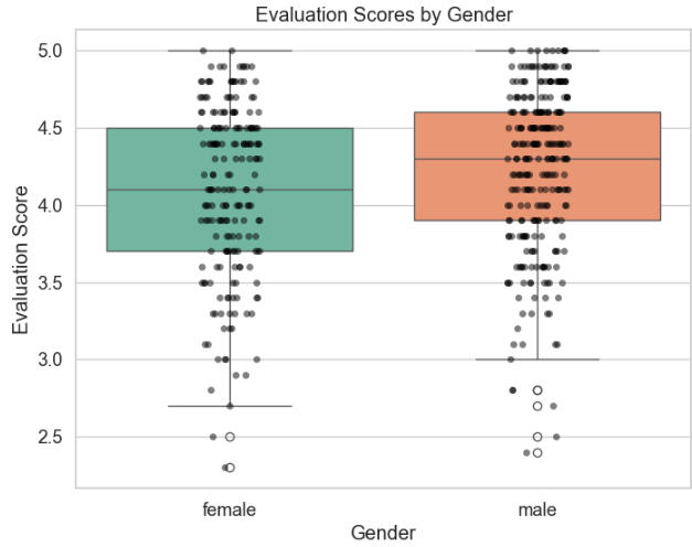
So we see that there is a difference, and that males seem to have higher evaluation scores. (Note that all three quartiles are higher for males.) Will a t-test support this conclusion?
So:H₀: Mean(male) ≤ Mean(female)
H₁: Mean(male) > Mean(female)
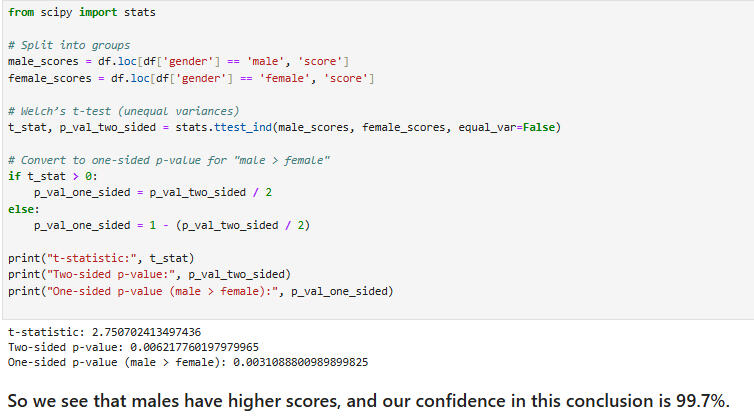
Results:
1. Beauty rating is more significant for male course evaluation scores.2. Males score higher in course evaluations than do females.Thu we have answered the questions initially posed.